Create an ecologically-organized heatmap using ggplot2 graphics

There are many useful examples of phyloseq heatmap graphics in the phyloseq online tutorials. In a 2010 article in BMC Genomics, Rajaram and Oono show describe an approach to creating a heatmap using ordination methods to organize the rows and columns instead of (hierarchical) cluster analysis. In many cases the ordination-based ordering does a much better job than h-clustering. An immediately useful example of their approach is provided in the NeatMap package for R. The NeatMap package can be used directly on the abundance table (otu_table-class) of phylogenetic-sequencing data, but the NMDS or PCA ordination options that it supports are not based on ecological distances. To fill this void, phyloseq provides the plot_heatmap() function as an ecology-oriented variant of the NeatMap approach to organizing a heatmap and build it using ggplot2 graphics tools. The distance and method arguments are the same as for the plot_ordination function, and support large number of distances and ordination methods, respectively, with a strong leaning toward ecology. This function also provides the options to re-label the OTU and sample axis-ticks with a taxonomic name and/or sample variable, respectively, in the hope that this might hasten your interpretation of the patterns (See the sample.label and taxa.label documentation, below). Note that this function makes no attempt to overlay hierarchical clustering trees on the axes, as hierarchical clustering is not used to organize the plot. Also note that each re-ordered axis repeats at the edge, and so apparent clusters at the far right/left or top/bottom of the heat-map may actually be the same. For now, the placement of this edge can be considered arbitrary, so beware of this artifact of this graphical representation. If you benefit from this phyloseq-specific implementation of the NeatMap approach, please cite both our packages/articles.

plot_heatmap(
  physeq,
  method = "NMDS",
  distance = "bray",
  sample.label = NULL,
  taxa.label = NULL,
  low = "#000033",
  high = "#66CCFF",
  na.value = "black",
  trans = log_trans(4),
  max.label = 250,
  title = NULL,
  sample.order = NULL,
  taxa.order = NULL,
  first.sample = NULL,
  first.taxa = NULL,
  ...
)

Arguments

physeq	(Required). The data, in the form of an instance of the phyloseq-class. This should be what you get as a result from one of the import functions, or any of the processing downstream. No data components beyond the otu_table are strictly necessary, though they may be useful if you want to re-label the axis ticks according to some observable or taxonomic rank, for instance, or if you want to use a UniFrac-based distance (in which case your physeq data would need to have a tree included).
method	(Optional). The ordination method to use for organizing the heatmap. A great deal of the usefulness of a heatmap graphic depends upon the way in which the rows and columns are ordered.
distance	(Optional). A character string. The ecological distance method to use in the ordination. See distance.
sample.label	(Optional). A character string. The sample variable by which you want to re-label the sample (horizontal) axis.
taxa.label	(Optional). A character string. The name of the taxonomic rank by which you want to re-label the taxa/species/OTU (vertical) axis. You can see available options in your data using rank_names(physeq).
low	(Optional). A character string. An R color. See ?colors for options support in R (there are lots). The color that represents the lowest non-zero value in the heatmap. Default is a dark blue color, "#000033".
high	(Optional). A character string. An R color. See colors for options support in R (there are lots). The color that will represent the highest value in the heatmap. The default is "#66CCFF". Zero-values are treated as NA, and set to "black", to represent a background color.
na.value	(Optional). A character string. An R color. See colors for options support in R (there are lots). The color to represent what is essentially the background of the plot, the non-observations that occur as NA or 0 values in the abundance table. The default is "black", which works well on computer-screen graphics devices, but may be a poor choice for printers, in which case you might want this value to be "white", and reverse the values of high and low, above.
trans	(Optional). "trans"-class transformer-definition object. A numerical transformer to use in the continuous color scale. See trans_new for details. The default is log_trans(4).
max.label	(Optional). Integer. Default is 250. The maximum number of labeles to fit on a given axis (either x or y). If number of taxa or samples exceeds this value, the corresponding axis will be stripped of any labels. This supercedes any arguments provided to sample.label or taxa.label. Make sure to increase this value if, for example, you want a special label for an axis that has 300 indices.
title	(Optional). Default NULL. Character string. The main title for the graphic.
sample.order	(Optional). Default NULL. Either a single character string matching one of the sample_variables in your data, or a character vector of sample_names in the precise order that you want them displayed in the heatmap. This overrides any ordination ordering that might be done with the method/distance arguments.
taxa.order	(Optional). Default NULL. Either a single character string matching one of the rank_names in your data, or a character vector of taxa_names in the precise order that you want them displayed in the heatmap. This overrides any ordination ordering that might be done with the method/distance arguments.
first.sample	(Optional). Default NULL. A character string matching one of the sample_names of your input data (physeq). It will become the left-most sample in the plot. For the ordination-based ordering (recommended), the left and right edges of the axes are adjaacent in a continuous ordering. Therefore, the choice of starting sample is meaningless and arbitrary, but it is aesthetically poor to have the left and right edge split a natural cluster in the data. This argument allows you to specify the left edge and thereby avoid cluster-splitting, emphasize a gradient, etc.
first.taxa	(Optional). Default NULL. A character string matching one of the taxa_names of your input data (physeq). This is equivalent to first.sample (above), but for the taxa/OTU indices, usually the vertical axis.
...	(Optional). Additional parameters passed to ordinate.

Value

A heatmap plot, in the form of a ggplot2 plot object, which can be further saved and modified.

Details

This approach borrows heavily from the heatmap1 function in the NeatMap package. Highly recommended, and we are grateful for their package and ideas, which we have adapted for our specific purposes here, but did not use an explicit dependency. At the time of the first version of this implementation, the NeatMap package depends on the rgl-package, which is not needed in phyloseq, at present. Although likely a transient issue, the rgl-package has some known installation issues that have further influenced to avoid making NeatMap a formal dependency (Although we love both NeatMap and rgl!).

References

Because this function relies so heavily in principle, and in code, on some of the functionality in NeatMap, please site their article if you use this function in your work.

Rajaram, S., & Oono, Y. (2010). NeatMap--non-clustering heat map alternatives in R. BMC Bioinformatics, 11, 45.

Please see further examples in the phyloseq online tutorials.

Examples

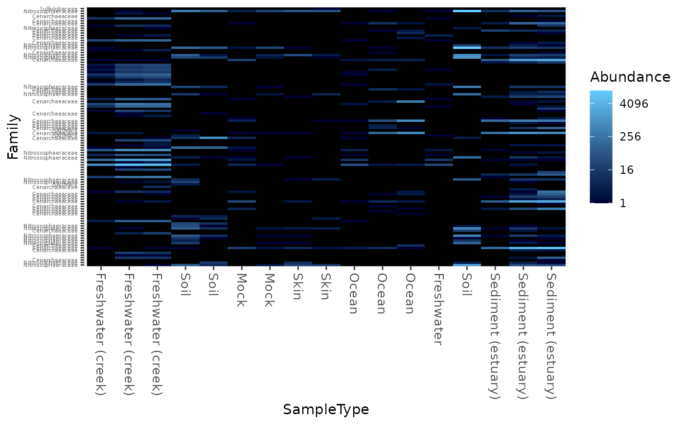
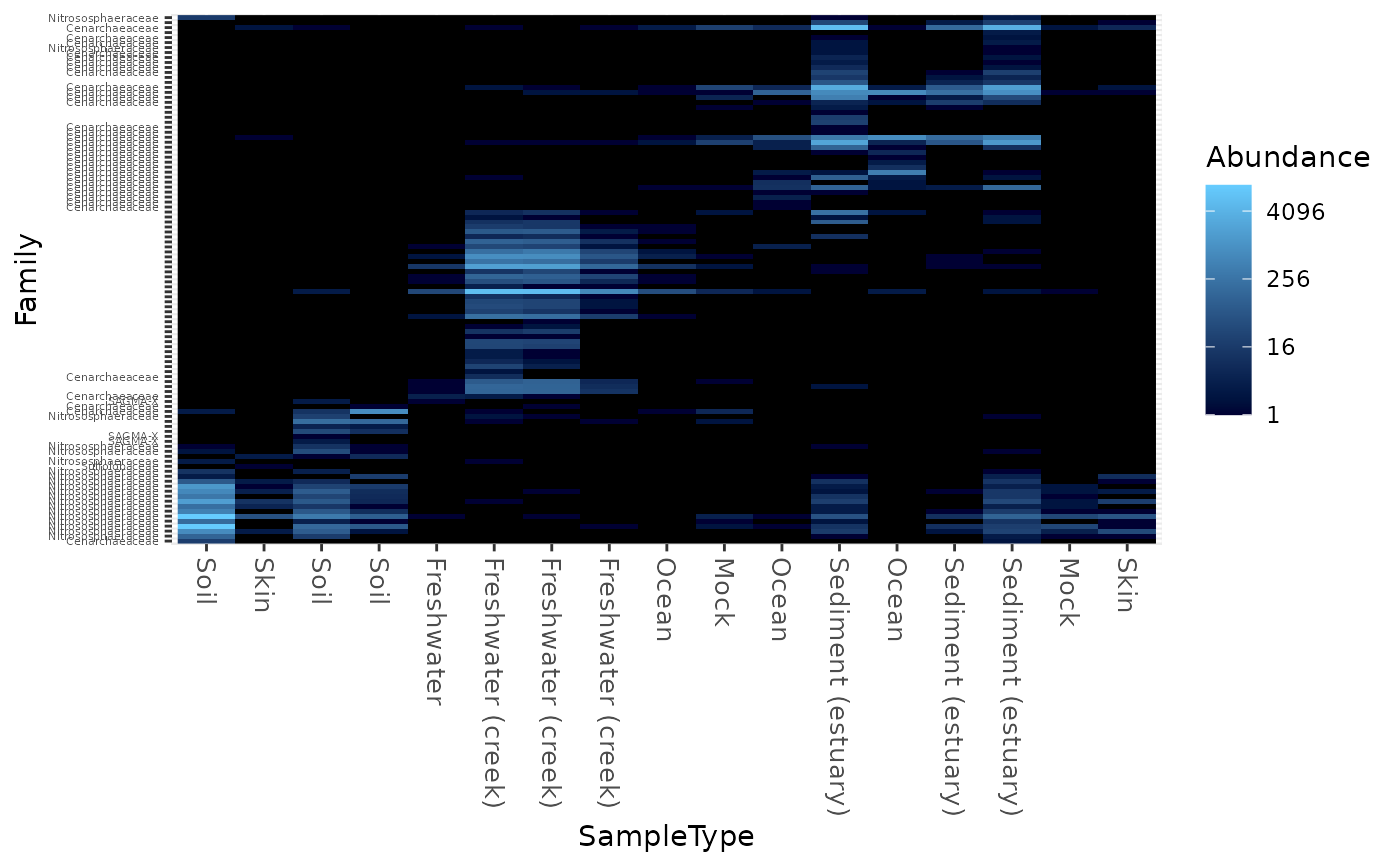
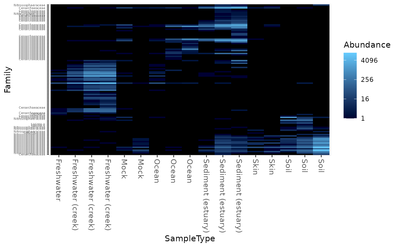
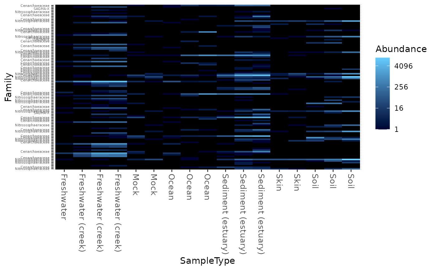
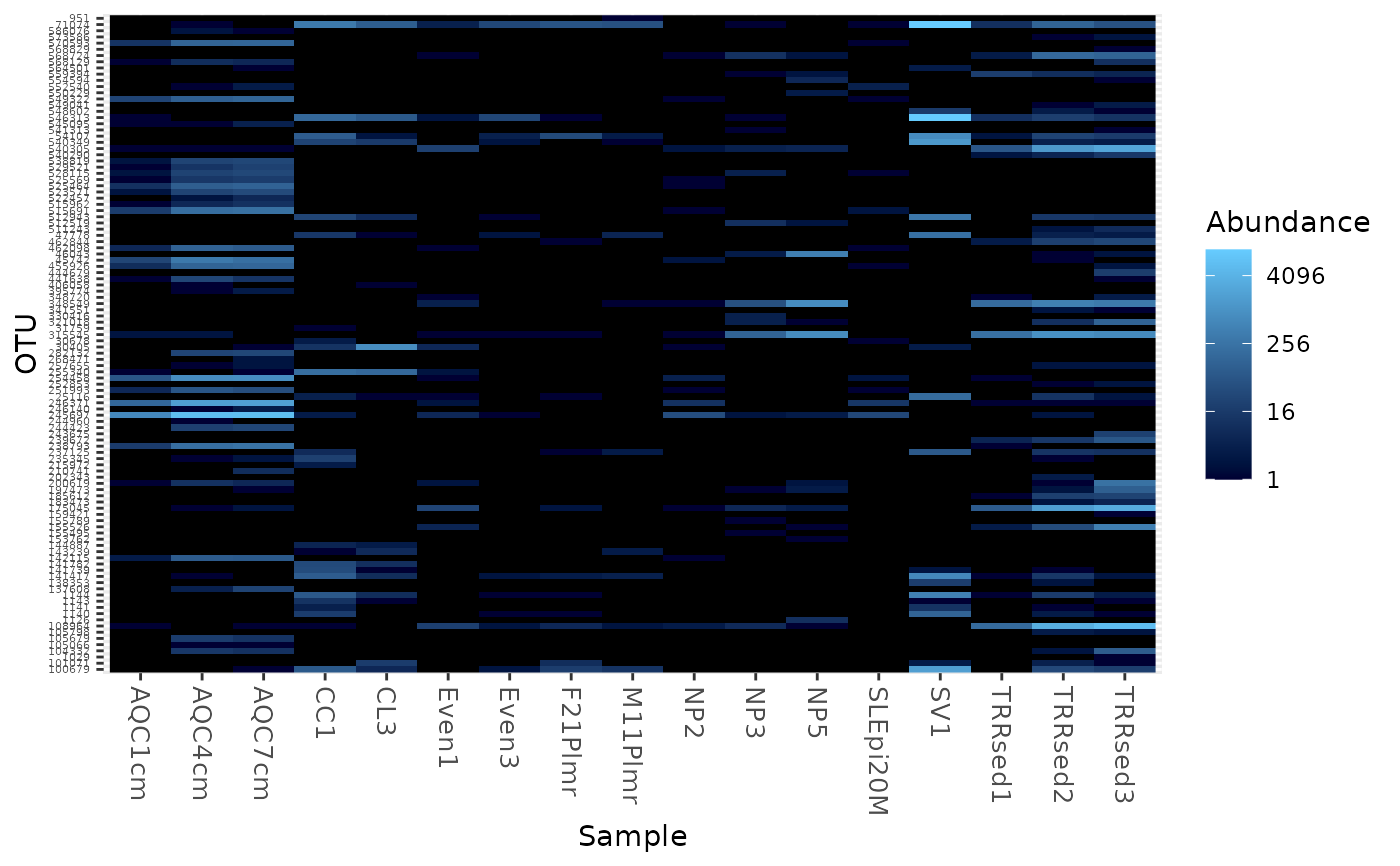
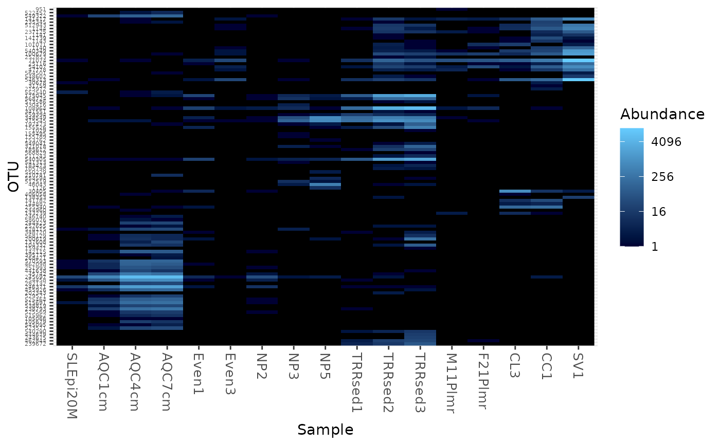
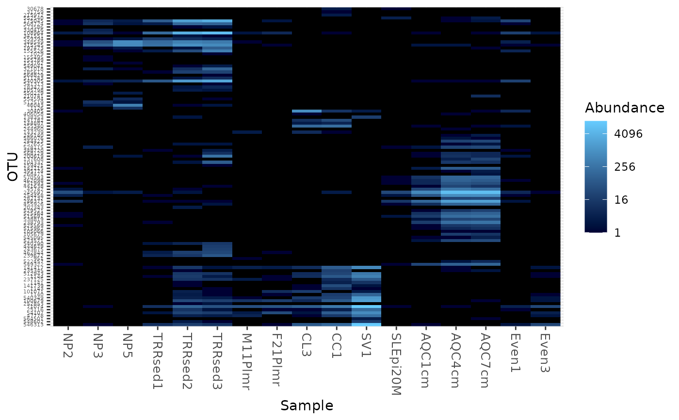
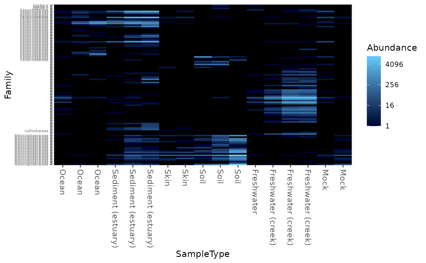
data("GlobalPatterns")
gpac <- subset_taxa(GlobalPatterns, Phylum=="Crenarchaeota")
# FYI, the base-R function uses a non-ecological ordering scheme,
# but does add potentially useful hclust dendrogram to the sides...
gpac <- subset_taxa(GlobalPatterns, Phylum=="Crenarchaeota")
# Remove the nearly-empty samples (e.g. 10 reads or less)
gpac = prune_samples(sample_sums(gpac) > 50, gpac)
# Arbitrary order if method set to NULL
plot_heatmap(gpac, method=NULL, sample.label="SampleType",
  taxa.label="Family")
#> Warning: Transformation introduced infinite values in discrete y-axis
# Use ordination
plot_heatmap(gpac, sample.label="SampleType", taxa.label="Family")
#> Warning: Transformation introduced infinite values in discrete y-axis
# Use ordination for OTUs, but not sample-order
plot_heatmap(gpac, sample.label="SampleType", taxa.label="Family",
  sample.order="SampleType")
#> Warning: Transformation introduced infinite values in discrete y-axis
# Specifying both orders omits any attempt to use ordination. The following
# should be the same.
p0 = plot_heatmap(gpac, sample.label="SampleType", taxa.label="Family",
  taxa.order="Phylum", sample.order="SampleType")
p1 = plot_heatmap(gpac, method=NULL, sample.label="SampleType",
  taxa.label="Family", taxa.order="Phylum", sample.order="SampleType")
#expect_equivalent(p0, p1)
# Example: Order matters. Random ordering of OTU indices is difficult to
# interpret, even with structured sample order
rando = sample(taxa_names(gpac), size=ntaxa(gpac), replace=FALSE)
plot_heatmap(gpac, method=NULL, sample.label="SampleType",
  taxa.label="Family", taxa.order=rando, sample.order="SampleType")
#> Warning: Transformation introduced infinite values in discrete y-axis
# # Select the edges of each axis. 
# First, arbitrary edge, ordering
plot_heatmap(gpac, method=NULL)
#> Warning: Transformation introduced infinite values in discrete y-axis
# Second, biological-ordering (instead of default ordination-ordering), but
# arbitrary edge
plot_heatmap(gpac, taxa.order="Family", sample.order="SampleType")
#> Warning: Transformation introduced infinite values in discrete y-axis
# Third, biological ordering, selected edges
plot_heatmap(gpac, taxa.order="Family", sample.order="SampleType",
  first.taxa="546313", first.sample="NP2")
#> Warning: Transformation introduced infinite values in discrete y-axis
# Fourth, add meaningful labels
plot_heatmap(gpac, sample.label="SampleType", taxa.label="Family",
  taxa.order="Family", sample.order="SampleType", first.taxa="546313",
  first.sample="NP2")
#> Warning: Transformation introduced infinite values in discrete y-axis