Agglomerate taxa using phylogeny-derived distances.

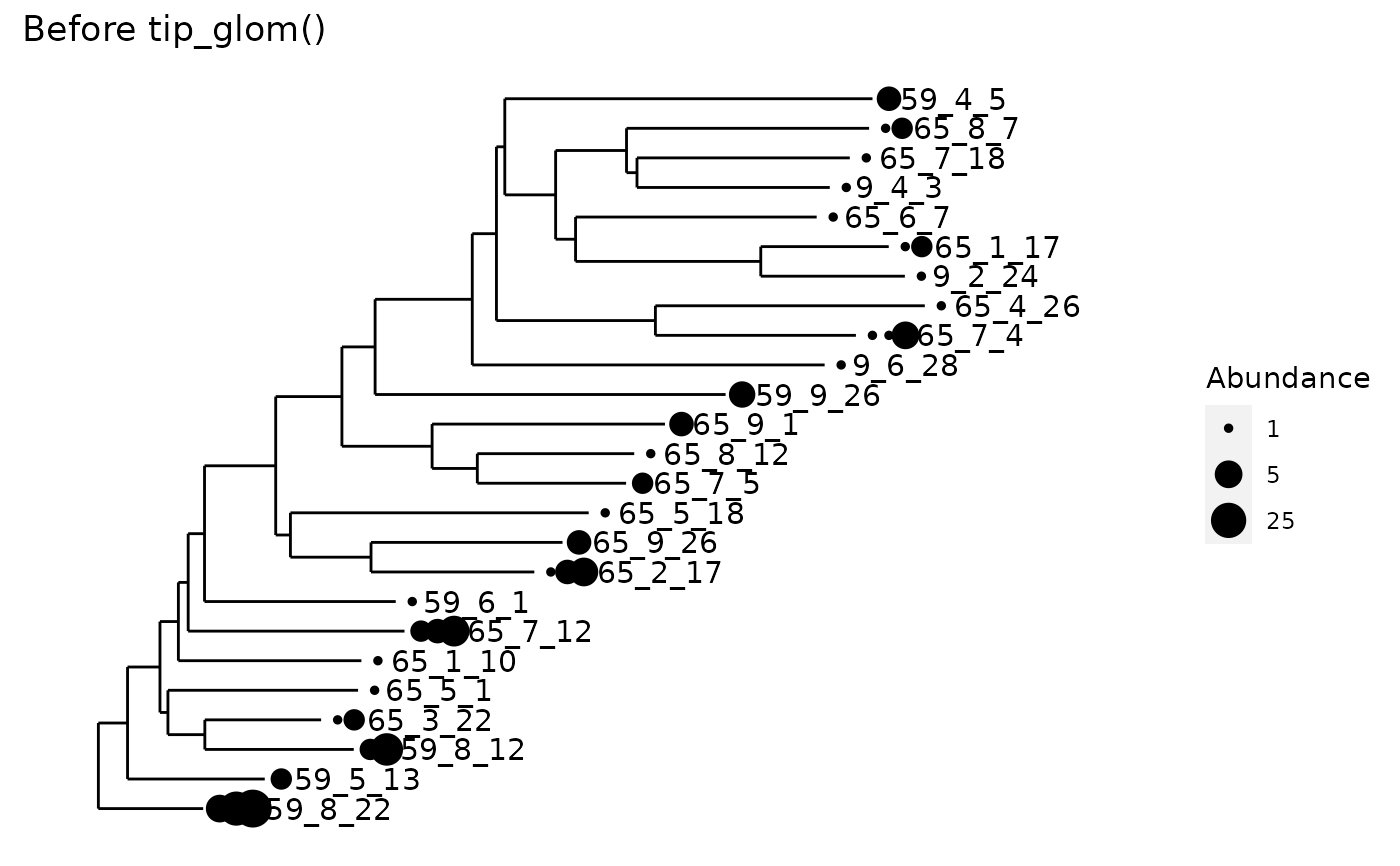
All tips of the tree separated by a phylogenetic cophenetic distance smaller than h will be agglomerated into one taxon.

tip_glom(physeq, h = 0.2, hcfun = cluster::agnes, tax_adjust = 1L, ...)

Arguments

physeq	(Required). A phyloseq-class(), containing a phylogenetic tree. Alternatively, a phylogenetic tree ape::phylo() will also work.
h	(Optional). Numeric scalar of the height where the tree should be cut. This refers to the tree resulting from hierarchical clustering of the distance matrix, not the original phylogenetic tree. Default value is 0.2.
hcfun	(Optional). A function. The (agglomerative, hierarchical) clustering function to use. The default is cluster::agnes() for phyloseq compatiblity.
tax_adjust	0: no adjustment; 1: phyloseq-compatible adjustment; 2: conservative adjustment (see merge_taxa_vec() for details)
...	(Optional). Additional named arguments to pass to hcfun.

Value

An instance of the phyloseq-class(). Or alternatively, a phylo() object if the physeq argument was just a tree. In the expected-use case, the number of OTUs will be fewer (see ntaxa()), after merging OTUs that are related enough to be called the same OTU.

Details

Can be used to create a non-trivial OTU Table, if a phylogenetic tree is available.

By default, simple "greedy" single-linkage clustering is used. It is possible to specify different clustering approaches by setting hcfun and its parameters in .... In particular, complete-linkage clustering appears to be used more commonly for OTU clustering applications.

The merged taxon is named according to the "archetype" defined as the the most abundant taxon (having the largest value of taxa_sums(physeq). The tree and refseq objects are pruned to the archetype taxa.

Speedyseq note: stats::hclust() is faster than the default hcfun; set method = "average" to get equivalent clustering.

Acknowledgements: Documentation and general strategy derived from phyloseq::tip_glom().

See also

phyloseq::tip_glom()

tree_glom() for direct phylogenetic merging

merge_taxa_vec()

cluster::agnes()

stats::hclust()

castor::get_all_pairwise_distances()

ape::phylo()

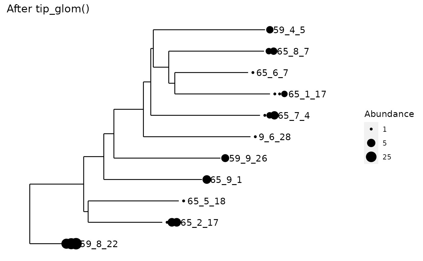
Examples

data("esophagus")
esophagus <- prune_taxa(taxa_names(esophagus)[1:25], esophagus)
plot_tree(esophagus, label.tips="taxa_names", size="abundance", 
  title="Before tip_glom()")
plot_tree(tip_glom(esophagus, h=0.2), label.tips="taxa_names", 
  size="abundance", title="After tip_glom()")

# *speedyseq only:* Demonstration of different `tax_adjust` behaviors
data(GlobalPatterns)

set.seed(20190421)
ps <- prune_taxa(sample(taxa_names(GlobalPatterns), 2e2), GlobalPatterns)

ps1 <- tip_glom(ps, 0.1, tax_adjust = 1)
#> Error in hcfun(dd, ...): unused argument (tax_adjust = 1)
ps2 <- tip_glom(ps, 0.1, tax_adjust = 2)
#> Error in hcfun(dd, ...): unused argument (tax_adjust = 2)
tax_table(ps1)[c(108, 136, 45),]
#> Error in h(simpleError(msg, call)): error in evaluating the argument 'object' in selecting a method for function 'tax_table': object 'ps1' not found
tax_table(ps2)[c(108, 136, 45),]
#> Error in h(simpleError(msg, call)): error in evaluating the argument 'object' in selecting a method for function 'tax_table': object 'ps2' not found