5 Solutions
5.1 Ratio-based relative DA analysis
Since bias creates constant fold errors (FEs) in the ratios among species, it can be countered by using DA methods that analyze fold differences (FDs) in these ratios. A variety of ratio-based methods have been developed under the framework of Compositional Data Analysis (CoDA; REFs). CoDA methods may more generally consider the ratios between products of multiple species, possibly raised to some exponent; a simple example is the geometric mean of several species. The mathematical operations of multiplication and exponentiation maintain constant FEs. Hence such products provide a method for aggregating species into a higher-level taxonomic units that maintains bias invariance when estimating FDs. Ratio-based analyses also avoid the potential for misinterpreting differences in a species’ proportion that are driven by the sum-to-one constraint (Gloor et al. (2017)).
We note two important caveats. First, in most MGS datasets, any given species is likely to be extremely rare in most samples, such that no sequencing reads are observed. In order to analyze FDs, DA methods interpret these zero counts as evidence that the true abundance of the species is very small (but still positive). A common approach to enable the computation of FDs in the presence of zeros is to add a small value, or ‘pseudo-count’, to the read counts, making all values positive. Unfortunately, this procedure violates bias invariance. How bias interacts with more sophisticated approaches for handling zeros remains an important open question. Second, the bias invariance of ratios among species does not extend to additive aggregates of species into higher-order taxa such phyla unless bias is conserved within the species group (McLaren, Willis, and Callahan (2019)). Multiplicative aggregates of species, recently used for biomarker discovery (Rivera-Pinto et al. (2018), Quinn and Erb (2020)), provide an alternative that remains bias-invariant but are harder to interpret.
If biological or technical considerations favor a DA method that is not bias invariant, it can be beneficial to also use a ratio-based method as a robustness check. For example, Hevroni et al. (2020) examined how the within-sample ranks of viral species changed from summer to winter. Since changes in within-sample ranks can be affected by bias, the authors also considered the changes in the centered log ratios (CLR) associated with each species. They found that the species whose within-sample ranks increased also increased in their CLR value, providing evidence that their initial results were not driven by bias.
5.2 Calibration using community controls
Community calibration controls are samples whose species identities and relative abundances are known, either by construction or by characterization with a chosen ‘gold standard’ or reference protocol (McLaren, Willis, and Callahan (2019), Clausen and Willis (2022)). Inclusion of these samples along with the primary samples in an MGS experiment can enable researchers to calibrate their MGS measurement by directly measuring and removing the effect of bias. Calibration can be extended to species not in the controls by imputing the efficiencies of the missing species using phylogenetic relatedness, genetic characteristics (such as 16S copy number), and/or phenotypic properties such as cell-wall structure.
Calibration makes it possible to correct for bias in relative and absolute DA methods that would otherwise not be bias invariant. To demonstrate, we used calibration to improve the estimated FDs between samples in the absolute abundance of a species in the bacterial mixtures from Brooks et al. (2015). We used the bias estimated from a single 7-species mixture to calibrate the MGS-derived proportions in all measured mixtures. We obtained calibrated absolute abundances by multiplying the calibrated proportions by the known total abundance (Equation (2.11)). Calibration greatly increased the accuracy of the estimated FDs (Figure 5.1, A vs. B). The fungal and vaginal case studies of Section 4 provide several practical examples of calibration in proportion-based DA analyses.
In studies of synthetic communities (like the fungal case study) or of ecosystems dominated by a relatively small number of culturable taxa (like the vaginal microbiome), calibration controls can be artificially constructed (‘mock’) communities. In other cases, natural community controls can be derived from aliquots of a homogenized microbiome sample. Measurement of these controls across multiple experiments enables characterization of the differential bias between experiments (McLaren, Willis, and Callahan (2019)). Calibration using differential bias can make results directly comparable across studies that used different protocols.
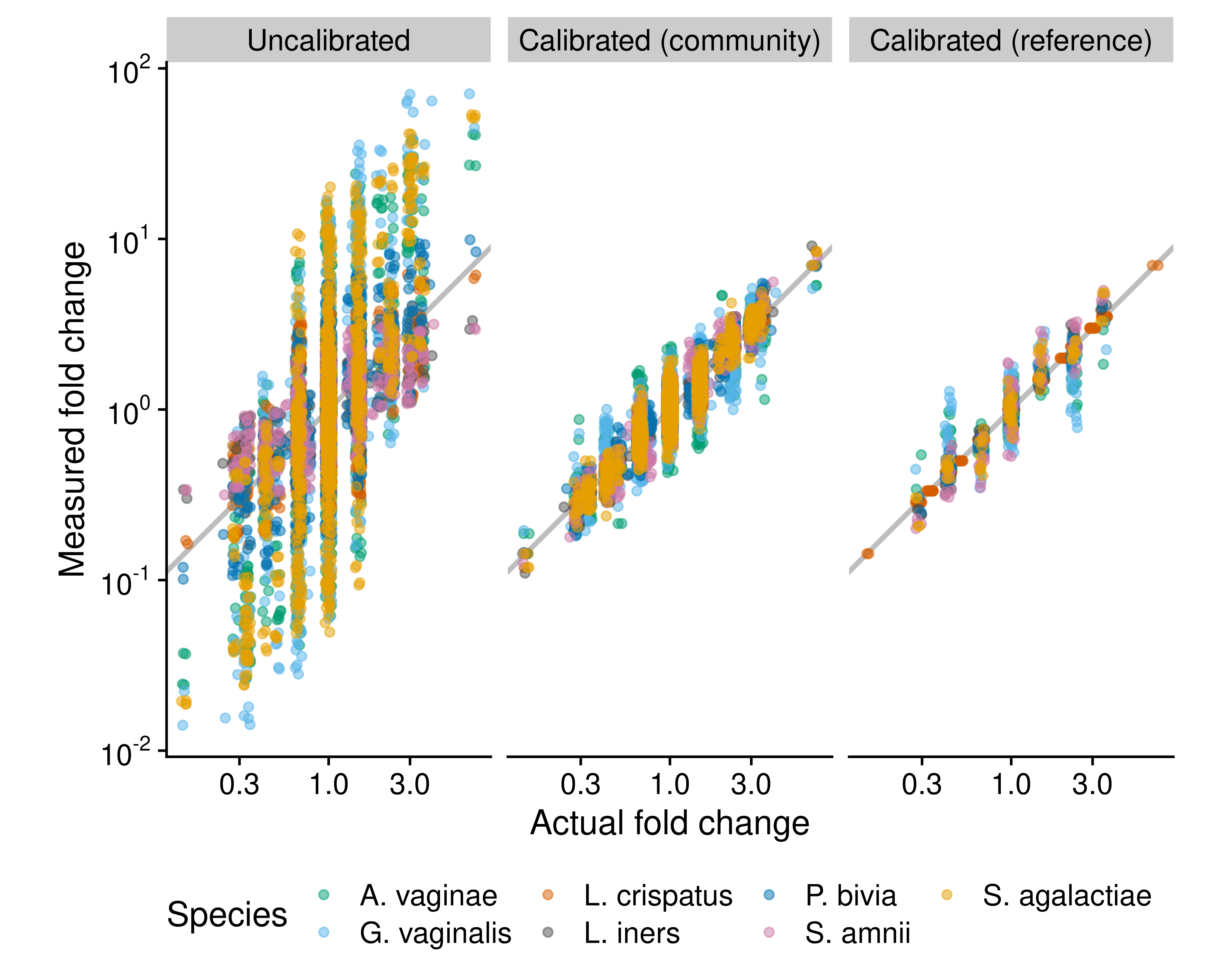
Figure 5.1: Fold differences can be calibrated using community controls or reference species. The figure compares the performance of three methods for measuring fold differences (FDs) in absolute cell density in cellular mock communities of 7 vaginal species, which were constructed and measured via 16S sequencing by Brooks et al. (2015). The ‘Uncalibrated’ FDs are derived directly from uncalibrated individual abundance measurements, which equal the product of the species’ proportion by the total density (which is constant by construction). The ‘Calibrated (community)’ measurements are computed from abundance measurements where the proportions are first corrected for the taxonomic bias that was estimated from a single sample that contained all 7 species. The ‘Calibrated (reference)’ measurements are computed from abundances measured with the reference-species method, with Lactobacillus crispatus used as the reference; that is, the true abundance of L. crispatus is treated as known and used to infer the abundance of the remaining 6 species. Only samples that contain L. crispatus are included.
5.3 Absolute-abundance methods with more stable FEs
There are many methods for obtaining absolute abundances from the relative abundances measured by MGS, but these methods have not previously been evaluated for their sensitivity to taxonomic bias (Williamson, Hughes, and Willis (2021) being a notable exception). Our theoretical results show that these methods differ in the extent to which taxonomic bias causes the FEs in species abundances to vary across samples. The effect of bias on absolute DA analysis can be mitigated by choosing methods with more stable FEs, using either of two general approaches.
5.3.1 Use complementary MGS and total-abundance measurements
A popular approach to measuring the absolute abundance of individual species is to multiply the species’ proportions from MGS by a measurement of the abundance of the total community (Equation (2.11)). The resulting species abundances are affected by taxonomic bias in the MGS and the total-abundance measurement (Equation (2.13)). Section 3 shows that the effect of both forms of bias on DA results can be reduced by choosing MGS and total-abundance methods that have similar taxonomic bias.
Consider the debate over whether flow cytometry or 16S qPCR are better methods for measuring total abundance for the purposes of normalizing 16S amplicon sequencing data (Galazzo et al. (2020), Jian, Salonen, and Korpela (2021)). Flow cytometry directly counts cells, whereas 16S qPCR measures the concentration of the 16S gene following DNA extraction. Thus the 16S qPCR measurement is subject to bias from extraction, copy-number variation, primer binding, and amplification, just like the 16S sequencing measurement. Although this shared bias likely makes 16S-qPCR less accurate as a measure of total cell concentration, our theory suggests that it will lead to more accurate FDs—and thus more accurate DA results.
More generally, these observations suggest that for the purposes of performing an absolute DA analysis from amplicon sequencing measurements, the ideal total-abundance measurement is qPCR of the same marker gene, from the same DNA extraction. Similar reasoning suggests that for shotgun sequencing, the ideal total-abundance measurement is bulk DNA quantification: Shotgun sequencing and bulk DNA quantification are both subject to bias from extraction and variation in genome size. Optimal use of these pairings requires thoughtful choices during bioinformatics. For example, performing copy-number correction on amplicon read counts prior to multiplication by qPCR measurements would be counter-productive, as it decouples bias in the two measurements. Additionally, the MGS proportions should be computed prior to discarding any unassigned reads, since species that are missing from the given taxonomy database still contribute to the total concentration of marker-gene and/or bulk DNA. Future experiments should evaluate the extent to which the taxonomic bias of DNA-based total-abundance measurements is stable across samples and shared with the complementary MGS measurement.
5.3.2 Normalize to a reference species
A second approach to obtaining absolute species abundances involves normalizing the MGS count for each species to that of a reference species with constant and/or known abundance (Equation (2.14)). Our theory predicts that taxonomic bias induces constant FEs in the abundances obtained by this approach, which will not affect DA results.
Previous studies have used species with a constant abundance as references: spike-ins, computationally-identified ‘housekeeping species’, and the host. Researchers may naturally be concerned about bias between the reference species and the native species being normalized against it (see, for example, Harrison et al. (2021)’s recommendations for spike-in experiments). Our results show that accurate FDs and DA results can be obtained so long as the relative efficiency of the focal species to the reference is consistent across samples. This condition is much weaker than requiring that bias is small (the relative efficiency is close to 1) and so greatly expands the applicability of spike-ins and host normalization in microbiome experiments.
Section 2.3 further proposed an additional class of reference species for normalizing MGS measurements: Species whose (absolute) abundance has been measured using a targeted method such as qPCR with species-specific primers. To demonstrate the ability for reference calibration to reduce error in FD measurements, we treated the abundance of one species (Lactobacillus crispatus) in the Brooks et al. (2015) mock community data as known, and used it to calibrate the abundances of all species. Doing so improved the resulting measurements of FDs in the abundance of all species (Figure 5.1). Direct, targeted measurement of a reference species removes the need for it to have a constant abundance, thus expanding the applicability of reference-species normalization to experiments where spike-ins or housekeeping species are not viable options. The targeted measurement need not itself be an unbiased measure of the reference species’ abundance; so long as it has constant FE, the abundances of native species obtained by normalization will also have constant FEs. In many ecosystems, there may not be a single universally-present species that can serve as a reference in all samples. Sample coverage can be increased by making targeted measurements of multiple species or of larger taxonomic groups; see Appendix REF for details.
5.4 Bias sensitivity analysis
Even if control measurements are not available, it is possible to computationally assess the sensitivity of a given DA result to taxonomic bias. A bias sensitivity analysis can be conducted by analyzing an MGS dataset multiple times under a range of possible taxonomic biases. First, a large number of hypothetical biases are generated from a user-specified probability distribution. Next, the DA analysis is re-run while using each simulated bias vector to calibrate the MGS measurements. This approach is highly flexible, and can be used to investigate the bias sensitivity of any DA method. Alternatively, existing DA methods can be extended to directly include the unknown taxonomic bias in their underlying statistical model, thereby providing DA estimates that inherently account for the added uncertainty in microbiome compositions due to the presence of unknown bias. (Greenland et al. (2005) compares these two approaches in a general context; Nixon et al. (2022) applies the second approach to microbiome data in the absence of taxonomic bias.)
Interpreting a bias sensitivity analysis is complicated by the large percentage of zero counts in species-level microbiome profiles, as the results may strongly depend on how these zeros are handled in the calibration process. Therefore it can be advantageous to jointly test the sensitivity of assumptions about zero-generating processes along with taxonomic bias, making statistical DA models that include bias and one or more zero-generating processes especially valuable. The development of tools and workflows to facilitate bias sensitivity analysis may provide an efficient way to increase scientists’ ability to assess the reliability of microbiome results, both for differential abundance and microbiome analyses more generally.
5.5 Bias-aware meta-analysis
Meta-analysis of microbiome samples measured across multiple studies must contend with the fact that different studies typically use different protocols and hence have different taxonomic biases. These different biases can be explicitly accounted for in a bias-aware meta-analysis which has the potential to improve statistical power as well as interpretability of multi-study DA analyses. Parametric meta-analysis models include study-specific latent parameters representing ‘batch effects’—non-biological differences in the data from each study which can distort the observed biological patterns. By estimating these ‘nuisance parameters’ along with the biological parameters of interest (such as the difference in a species’ log abundance between conditions), the meta-analysis aims to reduce statistical bias in the biological parameters created by the non-biological differences among studies (Leek et al. (2010),Wang and LêCao (2020)). In a bias-aware meta-analysis, the meta-analysis model is configured so that (some of) the latent parameters correspond to study- and species-specific relative efficiencies. If taxonomic bias is consistent within but not between studies, then this approach may improve the ability for the meta-analysis to accurately identify DA patterns as compared to meta-analysis methods in which the ‘batch effects’ do not reflect the multiplicative and compositional nature of taxonomic bias. The ability to infer and adjust for the differential bias between studies can be increased by measuring one or more shared control samples alongside the experiment-specific samples.