5 Potential solutions
The theoretical results from Section 3 suggest a number of potential methods to avoid, correct, or otherwise mitigate the errors created by taxonomic bias. We present five that seem particularly promising: The first three are methods to correct or otherwise account for the effects of taxonomic bias to obtain more accurate DA results, whereas the second two treat the measurement efficiencies as unknown parameters and seek to understand the additional uncertainty they create, either in the results of individual studies or in joint analysis of multiple studies that used different MGS protocols.
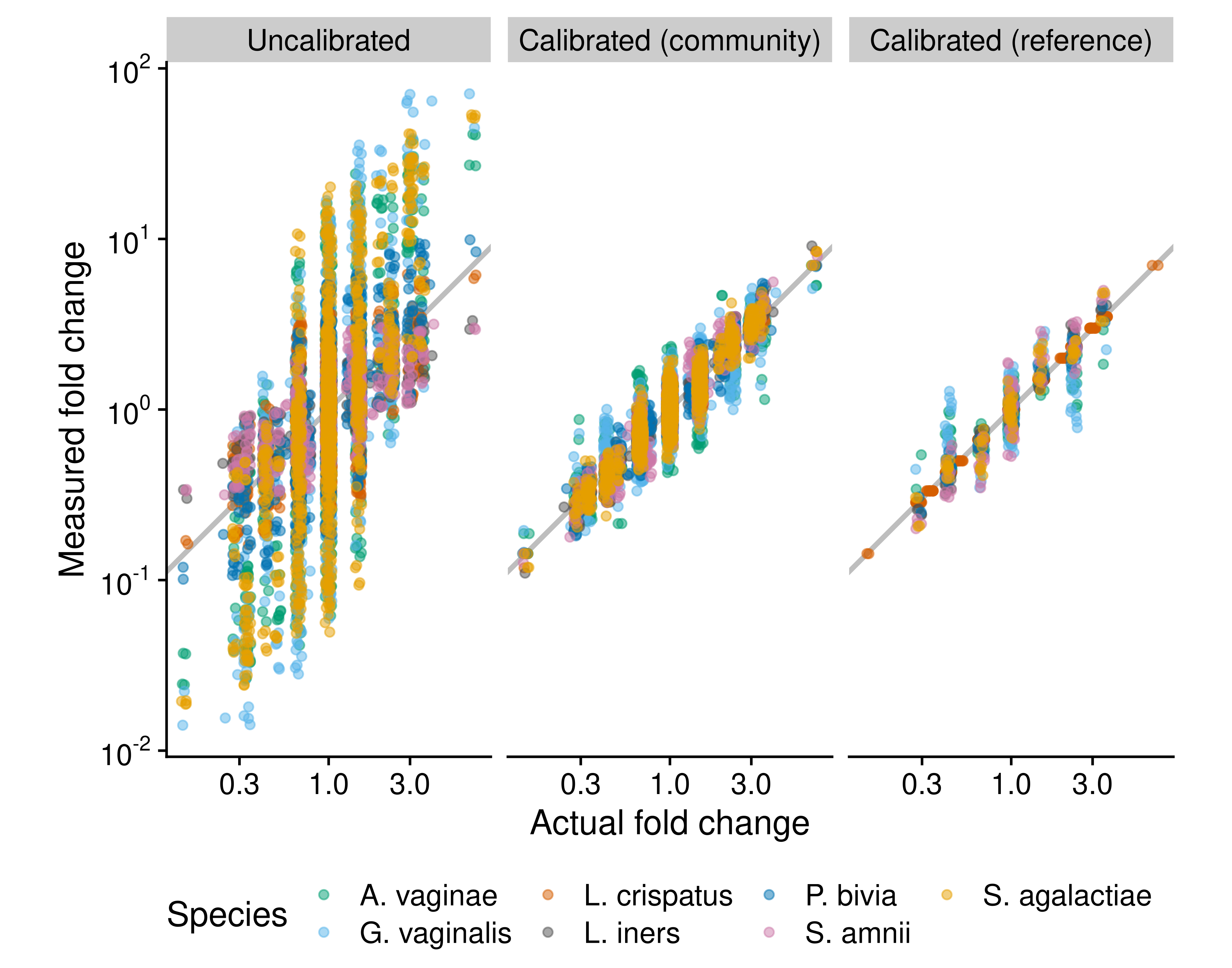
Figure 5.1: Fold changes can be calibrated using community controls or reference species. The figure compares the performance of three methods for measuring fold changes in absolute cell density in cellular mock communities of 7 vaginal species, which were constructed and measured via 16S sequencing by Brooks et al. (2015). The ‘Uncalibrated’ fold changes are derived directly from uncalibrated individual abundance measurements, which equal the product of the species’ proportion by the total density (which here is be known to be constant by construction). The ‘Calibrated (community)’ measurements are computed from abundance measurements where the proportions are first corrected for the taxonomic bias that was estimated from a single sample that contained all 7 species. The ‘Calibrated (reference)’ measurements are computed from abundances measured with the reference-species method, with Lactobacillus crispatus used as the reference; that is, the true abundance of L. crispatus is treated as known and used to infer the abundance of the remaining 6 species. Only samples that contain L. crispatus are included.
5.1 Calibrate compositions using community controls
The most complete but experimentally challenging approach to mitigating taxonomic bias involves directly measuring the efficiencies of individual species using control samples (McLaren, Willis, and Callahan (2019)). Suitable controls are any community sample whose composition (species identities and relative abundances) has been previously characterized, either by construction (in the case of constructed ‘mock’ communities) or by measurement with a reference protocol chosen to serve as a measurement standard. These controls, when measured alongside the target experimental samples, can be used to estimate the relative efficiencies among the superset of species across the control samples. The estimated efficiencies can then be used to calibrate the measured relative abundances among the control species in the target samples to the chosen measurement standard, by simply dividing the species’ read counts by their corresponding efficiencies (McLaren, Willis, and Callahan (2019)) or using a more sophisticated statistical modeling framework. These calibrated compositions can then be used for arbitrary downstream microbiome analyses, including DA analysis. Calibration of species not in the controls requires first imputing their efficiencies from the control measurements, for example using phylogenetic relationships, genetic characteristics (such as 16S copy number), and/or phenotypic properties (such as cell-wall structure). Though such imputation is conceptually straightforward, its accuracy and ultimate utility remain untested.
- The above states the approach; can add description/discussion of application to the MOMS-PI and Leopold and Busby (2020) cases and developments and challenges in availability of control communities
- ‘more sophisticated modeling framework’ - cite Williamson, Hughes, and Willis (2021) and https://microbiomemeasurement.org/posts/bias-estimation-from-mocks-with-fido/
5.2 Use ratio-based abundance measurement
The DA analyses we consider don’t need accurate estimates of relative abundances within individual samples—they only require accurate fold changes across samples. Section 3 showed that fold changes in species ratios and ratio-based density estimates can remain accurate even when taxonomic bias distorts the values in individual samples. Hence a solution is to use to analyze variation in ratios and ratio-based density estimates. For the latter, practical options include
- spike-ins of extraneous species at constant and/or known density
- housekeeping taxa, stipulated or computationally identified as having a constant density across samples
- targeted measurement of specific taxa
TBD what further discussion or illustration to have here.
5.3 Calibrate fold changes using measurements of targeted taxa
In some cases, we may still which to use a proportion-based approach to analyzing variation in density. For example, in some systems measuring total cell concentration may be easier than implementing a spike-in experiment or determining a set of reference species to directly measure for which at least one species is present in all samples. In this case, targeted measurements of one or more reference species can be used to validate and/or correct the fold changes or regression coefficients infered from the proportion-based densities. Recall that the error in proportion-based log fold changes (LFCs) is shared among species and is equal to the inverse LFC fold change in mean efficiency (Equations (3.1) and (3.3); Figure 3.1D). Consequently, an accurate LFC of one or more reference species can serve as a general validation or used to correct the LFCs of all species.
- Note: I may not correctly understand the next example, since I don’t yet see how this interpretation of Table 1 meshes with Figure 4
We illustrate this idea with an example from the study by Lloyd et al. (2020) described in Section 4, which estimated doubling times for various taxa from the measured log increase in cell density with burial time in marine sediments. The primary analysis, which used proportion-based density estimates, was supported by targeted measurements (qPCR) of 16S concentration for several bacterial and archeal taxa (CHECK). In Core 30, the doubling time estimated for the Archaeal phylum Bathyarchaeota was estimated to be 10.1 years (CHECK) using the proportion-based densities and 10.3 years by qPCR (Lloyd et al. (2020) Table 1 and Figure 4). These doubling times correspond to highly similar estimated slopes of log density per year of \(1/10.1 \approx 0.99\) and \(1/10.3\approx 0.97\). The difference between these slopes, \(\approx 0.02\), estimates the slope of the mean efficiency. It’s small value suggests little systematic variation in mean efficiency with burial time and hence little systematic bias in the estimated doubling times derived from the proportion-based density estimates. In this case, close agreement in the DA results across methods for a specific taxon suggests that variation in sample mean efficiency did not significantly distort the MGS-based results and hence provides a degree of validation for all taxa, not just the taxa with targeted measurements. (An important caveat for this example is that this analysis assumes consistent efficiencies at the higher taxonomic levels used for qPCR measurement and MGS analysis performed by Lloyd et al. (2020).) Here we compared summary statistics; however, in principle a joint statistical analysis of targeted and proportion-based density measurements would provide more statistical power to estimate and correct the effects of variation in the mean efficiency across samples and provide calibrated fold change and regression estimates for all taxa [APPENDIX].
5.4 Perform a bias sensitivity analysis
What can we do for experiments that have been conducted without control communities, targeted control measurements, or spike-ins? One approach is to conduct a bias sensitivity analysis to probe the extent and way in which the results of a DA analysis are sensitive to different possible taxonomic biases in our experiment.
A straightforward approach to bias sensitivity analysis is to use computer simulation to randomly generate efficiency vectors, each of which is used to calibrate the MGS measurements. These calibrated MGS measurements represent the true compositions under the hypothesized taxonomic bias. By re-running our DA analysis and comparing results across these simulated datasets, we can begin to understand how our initial results might be influenced by the strength and structure of the taxonomic bias in our experiment.
The simulated efficiency vectors may be generated to reflect certain hypotheses about bias in the given system. The utility of such simulations can increase the more we learn about the magnitude of bias in different systems and the taxonomic and protocol features that determine it. Future work in developing tools and methods for simulating efficiency vectors and performing bias sensitivity analyses could be a valuable way to assay and improve the reliability of microbiome results—for differential abundance and microbiome analyses more generally.
5.5 Use bias-aware meta-analysis
So far we have considered analysis of samples subject to the same taxonomic bias; however, meta-analysis of microbiome samples measured across multiple studies must often contend with a diversity of protocols and hence taxonomic biases in different groups of samples. This inconsistency in taxonomic bias across studies poses a problem even for ratio-based analyses where the effects of bias might cancel within a study.
A potential solution is to perform a bias-aware meta-analyses that jointly analyzes multiple data from studies while explicitely acknowledges the distinct, unknown taxonomic bias in each study. Parametric microbiome meta-analysis models already include sets of species-specific latent parameters to model “batch effects”—amorphous differences in the measurements of each study. By configuring these models so that these latent parameters correspond to the study and species specific efficiencies, we can increase the biological interpretability of these models and gain ability to determine whether disageements in DA results across studies are due to differences in taxonomic bias or other differences (such as host cohort or study design). Using a biophysically motivated model parameterization may also lead to performance gains in terms of increased explanatory power for a given model complexity, as seen for models of mock community measurements by McLaren, Willis, and Callahan (2019), which can increase improve our ability to find reproducible microbial associations in a given meta-study.
5.6 Supplemental figures

Figure 5.2: Example of a bias sensivity analysis.